Getting Started
This tutorial walks from installation to a first plot. It uses only the public surface that ships with v3.2.2: ddacs.load, ddacs.open_h5, ddacs.inspect_h5, and the visualization helpers.
The companion notebook at notebooks/01_getting_started.ipynb reproduces every cell below; open it side by side to run as you read.
1. Install
The PyTorch adapter is optional. Install it explicitly if a model is to be trained:
For hardware specific PyTorch builds (CUDA, ROCm, MPS) see pytorch.org and install PyTorch before ddacs.
Verify the install. From a Python REPL or notebook cell:
Or as a single shell command (handy on Linux servers where opening a REPL is overkill):
Output:
2. Download the sample bundle
The full dataset is large. For a first walkthrough, download the small bundle (~22 MB) from the repository root:
The command writes metadata.json, process_parameters.csv, and one sample simulation zip (258864.zip) into ./data/. The zips are not extracted; mlcroissant reads them in place.
If the notebook is launched from notebooks/, the same data directory resolves to ../data. Both point at the same place; pick the line that matches your working directory and comment out the other.
from pathlib import Path

DATA_DIR = Path('./data')      # repository root
# DATA_DIR = Path('../data')   # uncomment instead when running from inside notebooks/
sim_id   = 258864              # one bundled sample simulation
3. Load the dataset
ddacs.load(data_dir=...) returns an mlcroissant.Dataset. The default data_dir is ./data, so without an explicit argument the call assumes you are at the repository root.
ds = ddacs.load(data_dir=DATA_DIR)
print(ds.metadata.name)
print([rs.id for rs in ds.metadata.record_sets])
Output:
DDACS
['process-parameters', 'field-map', 'simulation-provenance',
 'springback-minimal', 'springback-prediction',
 'forming-snapshot', 'cutting-view']
The dataset is composed of named RecordSets. Each RecordSet defines a fixed selection of fields suitable for one task (e.g. springback prediction, forming snapshot).
4. Iterate records
The process-parameters RecordSet is the simulation index. It iterates 32,466 rows, one per simulation:
for n, rec in enumerate(ds.records('process-parameters'), start=1):
    if n == 1:
        for k, v in rec.items():
            print(f"{k:42s} = {v}")
    if n >= 1:
        break
Output (first row):
process-parameters/index                   = 16039
process-parameters/geometry                = b'rectangular'
process-parameters/curvature_radius        = 30.0
process-parameters/bottom_radius           = 5.0
process-parameters/wall_angle              = 10.0
process-parameters/material_scaling_factor = 0.9
process-parameters/sheet_metal_thickness   = 0.95
...
The springback-minimal RecordSet pulls real HDF5 arrays from the local zips. With the small bundle only the sample simulation is iterable; with the full download it produces 32,466 records.
5. Inspect one simulation
ddacs.open_h5(sim_id, data_dir=...) resolves the manifest, finds the right zip, reads the HDF5 member into memory and returns an h5py.File. It is read only and supports the with idiom:
Output:
['element_shell_bending_moment', 'element_shell_effective_plastic_strain',
 'element_shell_effective_plastic_strain_all_ipt', 'element_shell_ids',
 'element_shell_internal_energy', 'element_shell_node_ids',
 'element_shell_node_indexes', 'element_shell_normal_force',
 'element_shell_part_indexes', 'element_shell_shear_force',
 'element_shell_strain', 'element_shell_stress',
 'element_shell_stress_all_ipt', 'element_shell_stress_all_ipt_thickness',
 'element_shell_thickness', 'element_shell_unknown_variables',
 'node_acceleration', 'node_coordinates', 'node_displacement',
 'node_ids', 'node_velocity']
ddacs.inspect_h5 prints the group and dataset hierarchy of an open file or a path on disk:
Output (truncated; the full tree is in HDF5 structure):
258864.h5
├── @blankholder_force = 250000.0
├── @bottom_radius = 5.0
├── @geometry = concave
├── @sheet_metal_thickness = 0.99
├── OP10/
│   ├── blank/
│   │   ├── node_displacement  (4, 11236, 3) float64
│   │   ├── element_shell_thickness  (4, 11025) float64
│   │   └── ...
│   ├── binder/    (3 timesteps, no stress / thickness)
│   ├── die/       (3 timesteps, no stress / thickness)
│   ├── punch/     (3 timesteps, no stress / thickness)
│   └── general/   (global energies, per part metrics)
└── OP20/
    └── blank/    (2 timesteps)
Each line that starts with @ is an HDF5 attribute. Groups end in /; datasets show their shape and dtype.
6. First plot
The next cell renders the formed blank coloured by sheet thickness at the final OP10 timestep (after springback).
Three pieces of data are read from the HDF5 file:
nodes: node positions. The datasetOP10/blank/node_displacementhas shape(t=4, n_nodes, 3), one position per timestep; selecting[-1]keeps the configuration after springback.faces: element connectivity. The datasetOP10/blank/element_shell_node_indexeshas shape(n_elements, 4)because each shell is a quadrilateral of four node indices. There is no time axis: which nodes are connected by which element never changes during a simulation, so the array is read whole with[:].thickness: current shell thickness.OP10/blank/element_shell_thicknesshas shape(t=4, n_elements), again sliced with[-1]to match the post-springback state.
A note on three options that drive the plot:
FALSE_COLOR_CMAPis the false-colour diverging colormap: red at the lower bound, green at the centre, blue at the upper bound. Pairing it withvmin = nominal - delta,vmax = nominal + deltaplaces the green band on the nominal sheet thickness, so colour deviations immediately read as thinning (red) or thickening (blue).- Quarter symmetric model. OP10 only meshes one quadrant of the cup; the other three are implied by symmetry boundary conditions, so the file contains roughly 11 000 nodes covering a 100 mm x 100 mm patch. To render the full cup, pass
mirror=True, which reflects the mesh across thex = 0andy = 0planes and reverses the face winding on each reflection so the lighting stays consistent. - ISO 80000-2 axis labels : variables italic, units upright.
plot_meshapplies this automatically ($x$ in mm, etc.).
import matplotlib.pyplot as plt
import ddacs
from ddacs.visualization import FALSE_COLOR_CMAP

with ddacs.open_h5(sim_id, data_dir=DATA_DIR) as f:
    nodes     = f['OP10/blank/node_displacement'][-1]          # (n_nodes, 3) at final OP10 step
    faces     = f['OP10/blank/element_shell_node_indexes'][:]  # (n_elements, 4) : time invariant
    thickness = f['OP10/blank/element_shell_thickness'][-1]    # (n_elements,) at final OP10 step
    nominal   = float(f.attrs['sheet_metal_thickness'])         # 0.99 mm for this sim

half_range = 0.15
ax, cbar = ddacs.plot_mesh(
    nodes, faces,
    values=thickness,
    cmap=FALSE_COLOR_CMAP,
    vmin=nominal - half_range,
    vmax=nominal + half_range,
    colorbar_label='Thickness in mm',
    mirror=True,
)
plt.show()
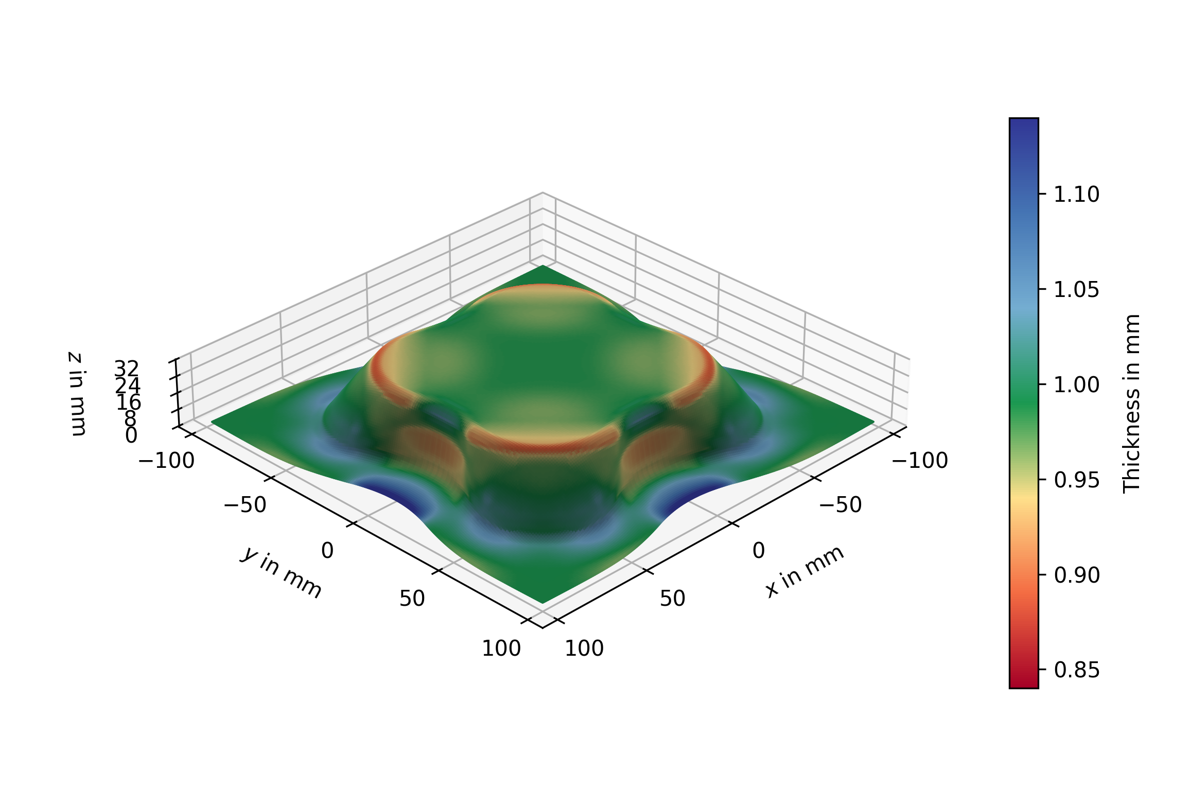
plot_mesh returns (ax, cbar): the matplotlib 3D axis and the colorbar. Both can be customised afterwards (e.g. ax.view_init(...) for a different camera angle, cbar.set_label(...) to change the label).
Where to go next
- Build your own view explains
ddacs.add_viewand the JSONPath transforms behind it. - PyTorch training covers
DDACSDataset, multi workerDataLoader, DDP, and the per simulation read benchmark. - Visualization covers mesh, point cloud, and vector field plotting in depth.
- Loose HDF5 recipe shows the CSV plus
h5py.Fileiteration loop for users who runddacs download --extract --remove-zip.