Streaming and numpy export

ddacs.streaming is the offline-iteration counterpart to DDACSDataset. It exists to solve two problems the published mlcroissant.Dataset.records(view) path does not:

1. Setup cost. records() walks every zip in the FileSet before yielding the first record, which takes several minutes on the full release. streaming.iter_view opens zips on demand and yields the first record in milliseconds.
2. Inner-loop training cost. Iterating an HDF5 view is bound by gzip decompression and h5py per-call overhead (~25 ms per record on NVMe, ~110 ms on HDD). For a 32 466-sim epoch this is the bottleneck. streaming.export_to_numpy walks the view once and writes flat .npy memmap shards; from then on the training loop reads records in microseconds via np.load(..., mmap_mode='r').

Both functions accept either the published Croissant views (springback-minimal, forming-snapshot, ...) or any custom view added with ddacs.add_view, via the dataset= kwarg.

The companion notebook at notebooks/06_streaming.ipynb reproduces every cell below.

import time
from pathlib import Path

import matplotlib.pyplot as plt
import numpy as np
import seaborn as sns

import ddacs

DATA_DIR      = Path('./data')     # repository root, or '../data' from notebooks/
EXPORT_DIR    = DATA_DIR / 'tutorial_export'
SAMPLE_SIM_ID = 258864             # bundled with `ddacs download --small`
ROCKET        = sns.color_palette('rocket', as_cmap=True)

1. Build a custom view

This is the same my-view shown in Build your own view: four representative field shapes, exposed as an in-memory mutation of the loaded ds. The published manifest on DaRUS is not modified.

ds = ddacs.load(data_dir=DATA_DIR)
ddacs.add_view(
    ds,
    'my-view',
    fields={
        'trajectory': ('op10_blank_node_displacement', None),       # all 4 timesteps
        'forming':    ('op10_blank_node_displacement', 2),          # one timestep
        'springback': ('op10_blank_node_displacement', [2, 3]),     # subset of timesteps
        'thickness':  'op10_blank_element_shell_thickness',         # whole field, shortcut form
    },
)

2. Preview one record with streaming.iter_view

ddacs.streaming.iter_view(view='my-view', dataset=ds) is the plain-Python counterpart to DDACSDataset.__iter__. No PyTorch dependency, no mlcroissant.Dataset.records() FileSet walk. It opens each zip on demand and yields one dict[str, np.ndarray] per simulation, with every alias already sliced according to its JSONPath transform.

for rec in ddacs.streaming.iter_view('my-view', data_dir=DATA_DIR, dataset=ds, sim_ids=[SAMPLE_SIM_ID]):
    for alias, value in rec.items():
        print(f'  {alias:12s} shape={value.shape}  dtype={value.dtype}')
    break

Output (with the small bundle on disk):

  trajectory   shape=(4, 11236, 3)  dtype=float64
  forming      shape=(11236, 3)  dtype=float64
  springback   shape=(2, 11236, 3)  dtype=float64
  thickness    shape=(4, 11025)  dtype=float64

Replace sim_ids=[SAMPLE_SIM_ID] with where=lambda row: row['rddac'] or simply omit both arguments to walk every simulation in process_parameters.csv.

The same function transparently handles both layouts: zipped (data_dir/h5/*.zip, the default) and loose (data_dir/h5/<sim_id>.h5, the layout after ddacs download --extract --remove-zip). Loose files take precedence when both contain the same simulation id.

3. Export to numpy with geometric normalisation

export_to_numpy walks the view once, applies any per-field or whole-record transforms, and writes each output alias into its own pre-allocated .npy memmap of shape (n_sims, *field_shape). It also writes sim_ids.npy so the row order is recoverable.

The record_transform below does three useful things at once and is a good template for the way training pipelines actually consume the dataset:

1. Normalise the point cloud geometry. ML point-cloud architectures (PointNet++, DGCNN, ...) almost always expect inputs in a unit cube. We centre forming on its centroid and scale by the largest absolute coordinate so the cloud lives in [-1, 1].
2. Derive the training target. The springback delta = springback[1] - forming is what a model would predict; precomputing it at export time avoids redoing the subtraction every epoch. Kept in physical mm so loss values stay interpretable.
3. Preserve the de-normalisation constants. The per-record center_mm (3-vector) and scale_mm (float) ride alongside the tensors so any downstream code can map a prediction back to physical mm without re-opening the HDF5 file.

transforms={alias: fn} would do the same on a single field; record_transform is the right tool when the output keys do not match the input keys, as here.

def normalize_and_emit(rec):
    """Centre+scale `forming` to [-1, 1] and derive the springback delta."""
    nodes  = rec['forming']                       # (n_nodes, 3) in mm
    center = nodes.mean(axis=0)                   # (3,) part centroid
    scale  = float(np.abs(nodes - center).max())  # half-extent along the dominant axis
    return {
        'forming':   ((nodes - center) / scale).astype(np.float32),  # in [-1, 1]
        'delta':     (rec['springback'][1] - nodes).astype(np.float32),  # mm, absolute
        'center_mm': center.astype(np.float32),
        'scale_mm':  np.float32(scale),
    }


paths = ddacs.streaming.export_to_numpy(
    'my-view',
    EXPORT_DIR,
    data_dir=DATA_DIR,
    dataset=ds,
    sim_ids=[SAMPLE_SIM_ID],
    record_transform=normalize_and_emit,
)
for alias, path in paths.items():
    size_kb = path.stat().st_size / 1024
    print(f'  {alias:10s} -> {path}   ({size_kb:7.1f} KB)')

Output:

  forming    -> ./data/tutorial_export/forming.npy   (  131.8 KB)
  delta      -> ./data/tutorial_export/delta.npy   (  131.8 KB)
  center_mm  -> ./data/tutorial_export/center_mm.npy   (    0.1 KB)
  scale_mm   -> ./data/tutorial_export/scale_mm.npy   (    0.1 KB)
  sim_ids    -> ./data/tutorial_export/sim_ids.npy   (    0.1 KB)

4. Read the shards back with load_export

ddacs.streaming.load_export(directory) opens the exported folder behind the standard Python data model (__len__, __getitem__, __iter__, plus by_sim_id). Each row is a plain dict[str, np.ndarray]. Reads are sub-millisecond after the first access and the full release fits even when it doesn't fit in RAM — only the rows you actually access are loaded from disk.

Why it is fast: memory-mapped reads in one paragraph (skip if not interested)

The shards are opened with mmap_mode='r', which maps each .npy file directly into the process's virtual address space. Accessing arr[i] becomes an ordinary memory read; the operating system fetches whatever page that lives on from disk on demand and keeps a copy in its page cache. No pickle, no buffer allocation, no copy on the read path. The same page cache is shared across processes, so a DataLoader(num_workers=N) does not multiply the cached data by N. Cold reads pay the disk seek + page fault; warm reads are RAM-fast.

load_export deliberately does not import torch. It just satisfies the same len + getitem protocol PyTorch's map-style Dataset uses, so the returned object plugs into DataLoader, tf.data.Dataset.from_generator, JAX, or a plain Python loop without any adapter. Pass fields=["forming", "delta"] to load a subset; unknown names raise ValueError so typos surface immediately.

The scalar metadata (center_mm, scale_mm) sits alongside the tensors at the same row index. That is the general pattern for storing custom per-record data alongside the tensors: anything that fits in a numpy array (scalar, vector, tensor, integer label, downsampled image, ...) can ride next to the main fields, declared by the record_transform. No separate metadata file required.

export = ddacs.streaming.load_export(EXPORT_DIR)

print(f'len(export)    = {len(export)}')
print(f'export.fields  = {export.fields}')
print(f'export.sim_ids = {export.sim_ids.tolist()}')

record = export[0]
for alias, value in record.items():
    print(f'  {alias:10s} shape={value.shape}  dtype={value.dtype}')

Output:

len(export)    = 1
export.fields  = ('center_mm', 'delta', 'forming', 'scale_mm')
export.sim_ids = [258864]
  center_mm  shape=(3,)  dtype=float32
  delta      shape=(11236, 3)  dtype=float32
  forming    shape=(11236, 3)  dtype=float32
  scale_mm   shape=()  dtype=float32

Round trip back to mm — inverting the normalisation is one numpy expression on the per-record data:

record = export[0]
forming_mm = record['forming'] * record['scale_mm'] + record['center_mm']
print(f'de-norm forming_mm range: [{forming_mm.min():+.3f}, {forming_mm.max():+.3f}] mm')

Output:

de-norm forming_mm range: [+0.000, +98.136] mm

For a PyTorch training loop, pass the same export straight into a DataLoader — the map-style Dataset protocol is just len + getitem, which this object provides natively:

from torch.utils.data import DataLoader
loader = DataLoader(export, batch_size=16, shuffle=True)

5. Time the two paths back to back

Both paths compute sum |delta| so we can verify numerical equality. With a single sim the absolute numbers are tiny, but the per-record ratio is what carries over to a full training loop: multiply by your epoch's n_sims to see the real win.

t0 = time.perf_counter()
stream_sum = 0.0
n = 0
for rec in ddacs.streaming.iter_view('my-view', data_dir=DATA_DIR, dataset=ds, sim_ids=[SAMPLE_SIM_ID]):
    stream_sum += float(np.abs(rec['springback'][1] - rec['forming']).sum())
    n += 1
t_stream = time.perf_counter() - t0

t0 = time.perf_counter()
mmap_sum = 0.0
m = 0
for record in export:
    mmap_sum += float(np.abs(record['delta']).sum())
    m += 1
t_mmap = time.perf_counter() - t0

print(f'iter_view   : {n} sim in {1000 * t_stream:.2f} ms  ({1000 * t_stream / n:.2f} ms/sim)')
print(f'load_export : {m} sim in {1000 * t_mmap:.2f} ms  ({1000 * t_mmap / m:.2f} ms/sim)')

Output (single sim on the HDD-backed bundle):

iter_view   : 1 sim in 370.03 ms  (370.03 ms/sim)
load_export : 1 sim in 0.37 ms  (0.37 ms/sim)

~1414x faster per record after a one-time ~470 ms export. The numerical results match to single-precision tolerance (sum |delta| identical between the two paths).

6. Visualise a sample

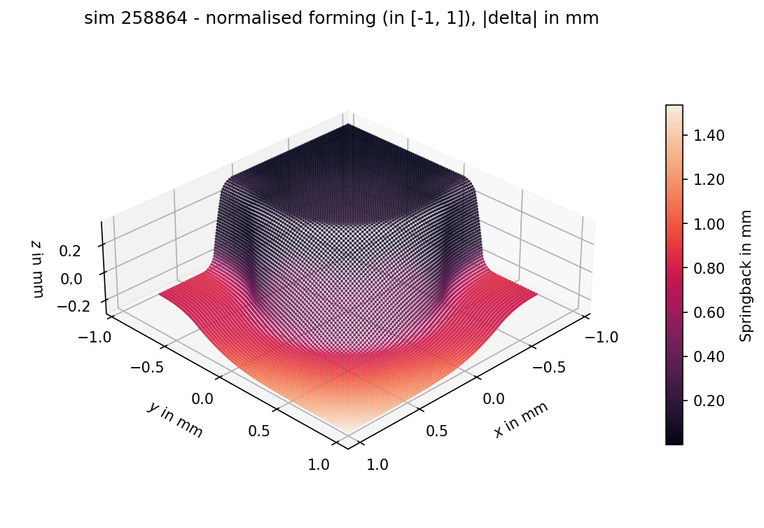
The shards are just numpy memmaps now, so looking at one record needs no view machinery: pick row 0, render its forming point cloud (already in [-1, 1] after the record_transform), colour it by |delta| in physical mm.

mirror=False here because the normalisation centred the part on the origin, and ddacs.plot_point_cloud's mirror flag assumes the input lives in the positive quadrant (raw OP10 coordinates in mm). On normalised data the four reflections overlay each other on the origin and produce a visual mess. To recover the full part in mm, multiply by scale_mm[i] and add center_mm[i] first (the forming_mm round trip from step 4) and then pass mirror=True.

sample_idx       = 0
sample_forming   = forming[sample_idx]
sample_magnitude = np.linalg.norm(delta[sample_idx], axis=1)

ax, cbar = ddacs.plot_point_cloud(
    sample_forming,
    values=sample_magnitude,
    cmap=ROCKET,
    colorbar_label='Springback in mm',
    mirror=False,
)
plt.show()

7. When records have variable shapes (export_to_numpy_per_sim)

export_to_numpy pre-allocates one memmap per alias, sized from record 0 as (n_sims, *field_shape). Every subsequent record must produce the exact same shape per alias; a shape mismatch raises a ValueError pointing here. The constraint is the right contract for views where every simulation has the same topology — e.g. the forming point cloud above, or any view that ran through a uniform sampling step that pinned N to a fixed value. It is not the right contract for views whose outputs vary across simulations: a graph view that exposes edge_index with sim-dependent edge counts, or a raw vertex set whose N differs per geometry corner.

For those cases, use ddacs.streaming.export_to_numpy_per_sim. Same iteration pipeline (iter_view + per-field transforms + whole-record record_transform), same _sim_id enrichment, but the writer is one np.savez(<sim_id>.npz) per record instead of one memmap per alias. Each .npz carries all the aliases for one simulation; consumers reload via np.load(path) and access by key.

ddacs.streaming.export_to_numpy_per_sim(
    "graph-view",
    "./data/graph_export",
    dataset=ds,
    record_transform=my_compose_chain,
    compressed=False,   # True for np.savez_compressed (smaller, slower load)
)

Trade-offs vs export_to_numpy:

• No memmap layout. Each load deserialises a small zip via numpy. For ~10 MB sims that is still sub-millisecond warm, but it loses the OS-page-cache sharing across DataLoader workers that export_to_numpy gets for free.
• No fixed-shape constraint. Variable-N and ragged tensors are fine.
• One file per sim. Random access by sim id is just np.load(out_dir / f"{sim_id}.npz").

Two ways to make a variable-shape view fit export_to_numpy instead — preferable when the data permits, because the mmap path is faster:

1. Sample to a fixed point count before export. A uniform / area-weighted barycentric sample (e.g. 4096 points per blank, 2048 per tool) gives every record the same shape per alias.
2. Pad to a max shape and emit a mask. Cheaper to write than to compose; wastes 20-30% of disk if the largest sim is much bigger than the median.

If neither fits, export_to_numpy_per_sim is the honest answer.

A minimal random-vertex sampler that pads or truncates every record to a fixed point count:

def uniform_sample(rec, n_points=4096, seed=0):
    rng = np.random.RandomState(seed)
    n_in = rec["forming"].shape[0]
    idx = rng.choice(n_in, n_points, replace=n_in < n_points)
    return {**rec, "forming": rec["forming"][idx], "delta": rec["delta"][idx]}

def chained(rec):
    return uniform_sample(normalize_and_emit(rec))

Pass chained as the record_transform=; the downstream export_to_numpy call now succeeds with forming and delta shaped (n_points, 3) in every record. The example above is naive — it samples vertex indices uniformly, ignoring triangle area, which under-represents large faces. Use it as a baseline; area-weighted barycentric sampling that respects mesh geometry is a separate concern beyond this tutorial.

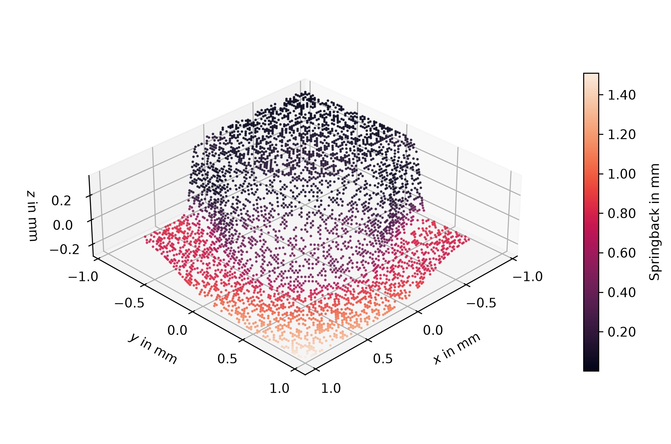
Same simulation rendered from the downsampled export: 4096 points instead of 11236, identical render code. The sparser sampling is visible but the springback gradient is preserved.

Where to go next

• The same transforms / record_transform pattern is exactly how you turn a categorical column (e.g. geometry='rectangular') into a small-int label: transforms={'geometry': lambda v: {'rectangular': 0, 'concave': 1, 'convex': 2}[v.decode()]}.
• streaming.iter_view is independent of the storage layout: it transparently reads loose h5/<sim_id>.h5 files (after ddacs download --extract --remove-zip) and zipped h5/*.zip archives. Loose files take precedence when both exist.
• For batched, sharded training there is DDACSDataset (PyTorch), which uses the same view-driven mechanics and benefits from the same add_view mutations via its dataset= kwarg.