Visualization
ddacs.plot_mesh, ddacs.plot_point_cloud, ddacs.plot_vectors, and ddacs.plot_2d_projection accept numpy arrays. Pair them with ddacs.open_h5 to read the arrays from a single simulation and render them. Every helper supports a mirror flag that reconstructs the full part from the quarter-symmetric model, and uses ISO 80000-2 axis labels (variables italic, units upright).
The companion notebook at notebooks/04_visualization.ipynb reproduces every cell below.
import matplotlib.pyplot as plt
import numpy as np
import seaborn as sns
import ddacs
from ddacs.visualization import FALSE_COLOR_CMAP, COMPONENT_COLORS

from pathlib import Path
DATA_DIR = Path('./data')      # repository root, or Path('../data') from notebooks/
sim_id   = 258864

ROCKET = sns.color_palette('rocket', as_cmap=True)
1. Thickness mesh
The blank ships with both initial coordinates (node_coordinates) and per-timestep positions (node_displacement[t]). Plotting the formed state means using node_displacement[-1] together with element_shell_thickness[-1] so geometry and colour map come from the same timestep.
Three choices drive the plot:
FALSE_COLOR_CMAP: diverging red -> green -> blue. Withvmin = nominal - delta,vmax = nominal + delta, green falls on the nominal sheet thickness, so deviations read as thinning (red) or thickening (blue).mirror=True: the simulation models a quarter of the cup by symmetry; mirroring acrossx = 0andy = 0reconstructs the full part.- ISO 80000-2 axis labels (variables italic, units upright) are applied automatically.
with ddacs.open_h5(sim_id, data_dir=DATA_DIR) as f:
    nodes     = f['OP10/blank/node_displacement'][-1]
    faces     = f['OP10/blank/element_shell_node_indexes'][:]
    thickness = f['OP10/blank/element_shell_thickness'][-1]
    nominal   = float(f.attrs['sheet_metal_thickness'])

half_range = 0.15
ax, cbar = ddacs.plot_mesh(
    nodes, faces,
    values=thickness,
    cmap=FALSE_COLOR_CMAP,
    vmin=nominal - half_range,
    vmax=nominal + half_range,
    colorbar_label='Thickness in mm',
    mirror=True,
)
plt.show()
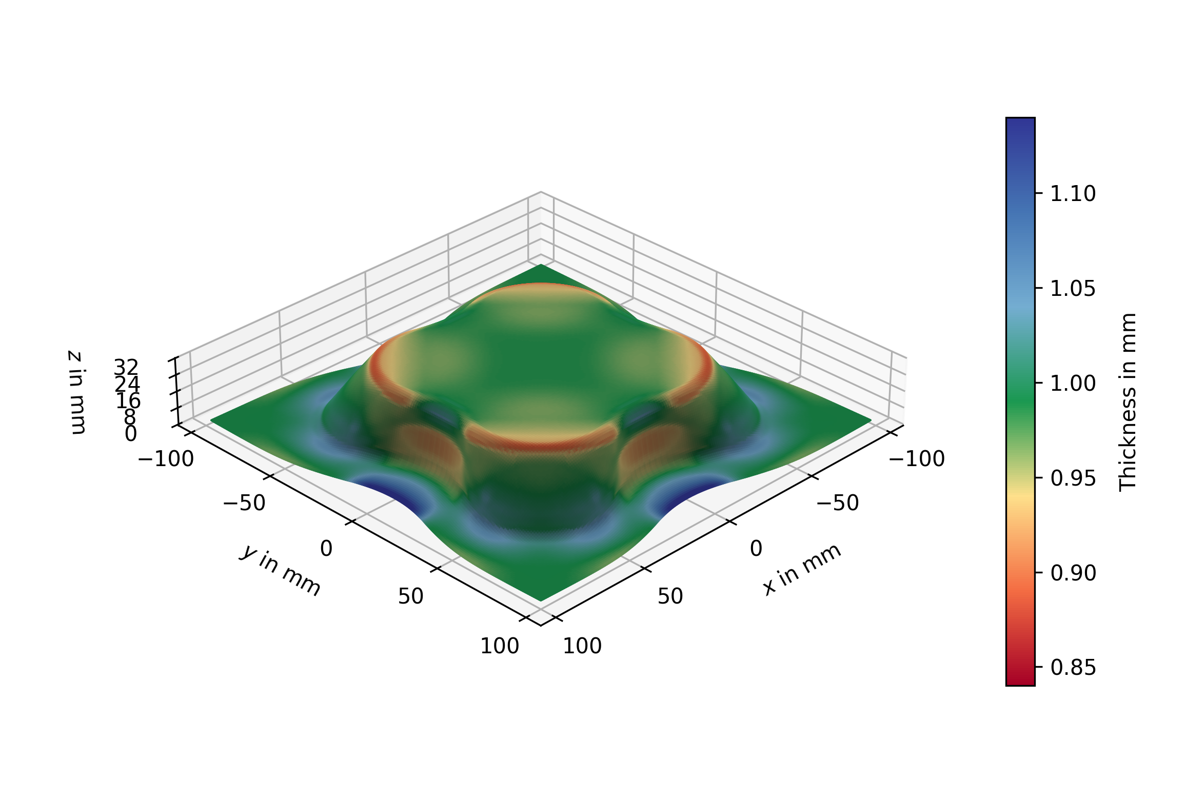
2. Component meshes in a 2 x 2 grid
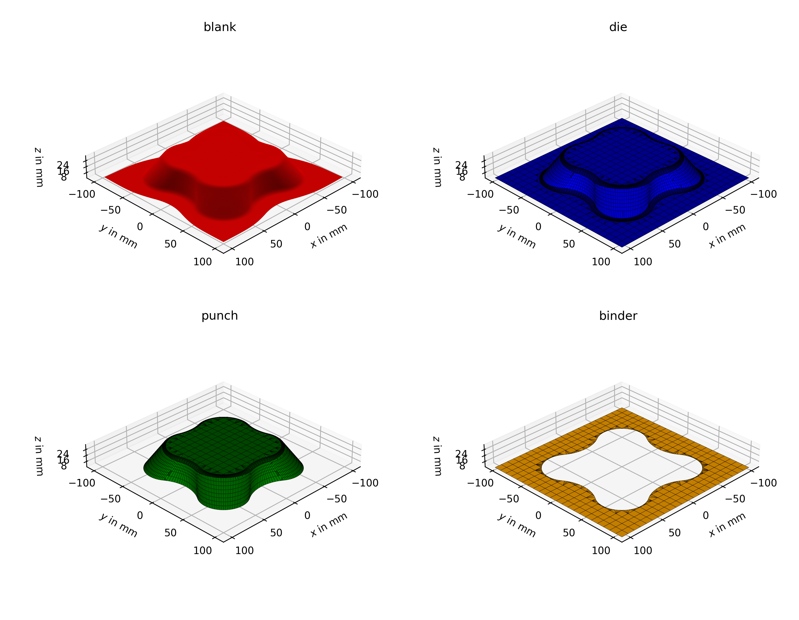
OP10 stores positions and shell connectivity for all four components. The face indices in element_shell_node_indexes are global: they index into the concatenation of all components' nodes, so each component's own slice starts at an offset. Subtracting face_idx.min() per component recovers valid local indices into the component's node_displacement array.
Three knobs drive the frame:
MIRROR: whenTrue, each subplot usesxlim/ylim = (-xmax, xmax) / (-ymax, ymax); whenFalse, the data stays in one quadrant so the limits start at0.PAD_XY = 1.15: the die and binder are a few mm wider than the blank in xy, so the blank-derived limits are padded outward by 15 % to keep them inside the frame.set_box_aspect((dx, dy, dz)): using data spans (not(1, 1, 1)) preserves the honest cup-vs-tool proportions; the binder is correctly flat atz = 0.
The three tools are rendered with a black wireframe to make the mesh density visible; the blank stays mono-coloured since the smooth shading reads cleaner against the workpiece colour.
with ddacs.open_h5(sim_id, data_dir=DATA_DIR) as f:
    parts = {
        name: (
            f[f'OP10/{name}/node_displacement'][-1],
            f[f'OP10/{name}/element_shell_node_indexes'][:],
        )
        for name in COMPONENT_COLORS
    }

MIRROR  = True
PAD_XY  = 1.15

blank_nodes = parts['blank'][0]
zmin = float(blank_nodes[:, 2].min())
zmax = float(blank_nodes[:, 2].max())
if MIRROR:
    xmax = float(np.abs(blank_nodes[:, 0]).max()) * PAD_XY
    ymax = float(np.abs(blank_nodes[:, 1]).max()) * PAD_XY
    xlim, ylim = (-xmax, xmax), (-ymax, ymax)
else:
    xlim = (0, float(blank_nodes[:, 0].max()) * PAD_XY)
    ylim = (0, float(blank_nodes[:, 1].max()) * PAD_XY)
zlim       = (zmin, zmax)
box_aspect = (xlim[1] - xlim[0], ylim[1] - ylim[0], zmax - zmin)

fig, axes = plt.subplots(
    2, 2,
    figsize=(11, 8),
    subplot_kw={'projection': '3d'},
    constrained_layout=True,
)

for ax, name in zip(axes.flat, COMPONENT_COLORS):
    nodes, faces = parts[name]
    faces = faces - faces.min()        # global -> local indices
    edgecolor = COMPONENT_COLORS[name] if name == 'blank' else 'black'
    ddacs.plot_mesh(
        nodes, faces,
        ax=ax,
        facecolors=COMPONENT_COLORS[name],
        edgecolors=edgecolor,
        linewidth=0.2,
        mirror=MIRROR,
    )
    ax.set_title(name)
    ax.set_xlim(xlim)
    ax.set_ylim(ylim)
    ax.set_zlim(zlim)
    ax.set_box_aspect(box_aspect)

fig.text(0.0, 0.0, " ")  # reserve a left margin so z-labels are not clipped
plt.show()
3. Springback magnitude
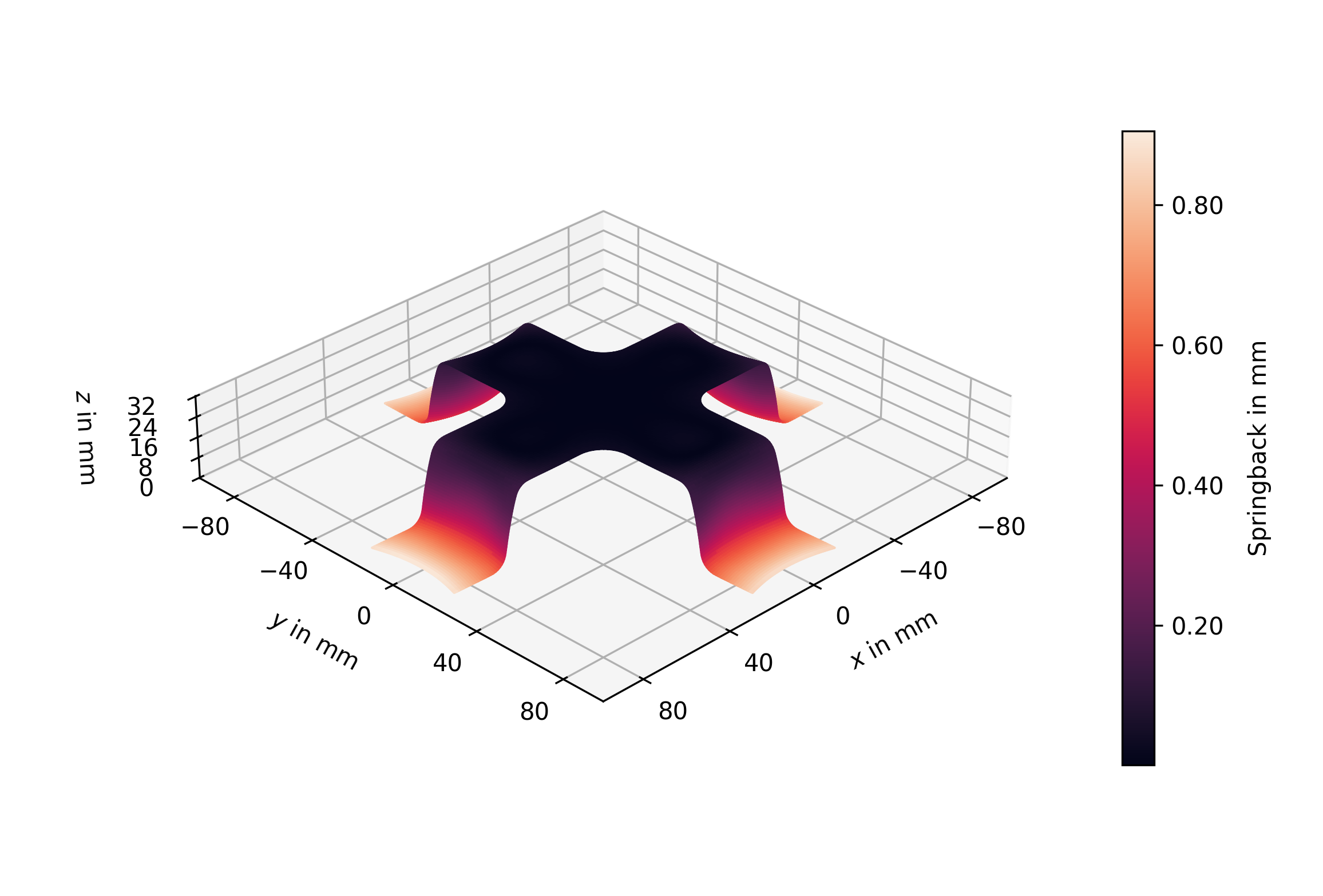
Springback is the elastic recovery of the workpiece after the tools release. Once the load is removed, the part partially snaps back towards its original geometry and a residual displacement field remains. It is the dominant geometric error in stamping and the standard target for ML models trained on this dataset.
OP20 stores two blank timesteps: the state immediately after cutting (still under contact) and the relaxed state after springback. The per-node delta pos[-1] - pos[-2] is the springback vector; its magnitude |delta| is the standard scalar field for "how much did this node move?". Plotting it on the OP20 mesh (rocket cmap from seaborn) shows where the part deforms most strongly on the actual surface. shade=False removes the per-face lighting so each face's rendered colour matches the colorbar exactly.
with ddacs.open_h5(sim_id, data_dir=DATA_DIR) as f:
    pos     = f['OP20/blank/node_displacement'][:]
    faces20 = f['OP20/blank/element_shell_node_indexes'][:]

displacement   = pos[-1] - pos[-2]
magnitude      = np.linalg.norm(displacement, axis=1)
# plot_mesh expects per-face values; average the per-node magnitude over each face.
face_magnitude = magnitude[faces20.astype(np.int64)].mean(axis=1)

ax, cbar = ddacs.plot_mesh(
    pos[-1], faces20,
    values=face_magnitude,
    cmap=ROCKET,
    vmin=float(magnitude.min()),
    vmax=float(magnitude.max()),
    colorbar_label='Springback in mm',
    mirror=True,
    shade=False,
)
plt.show()
4. Springback vector field
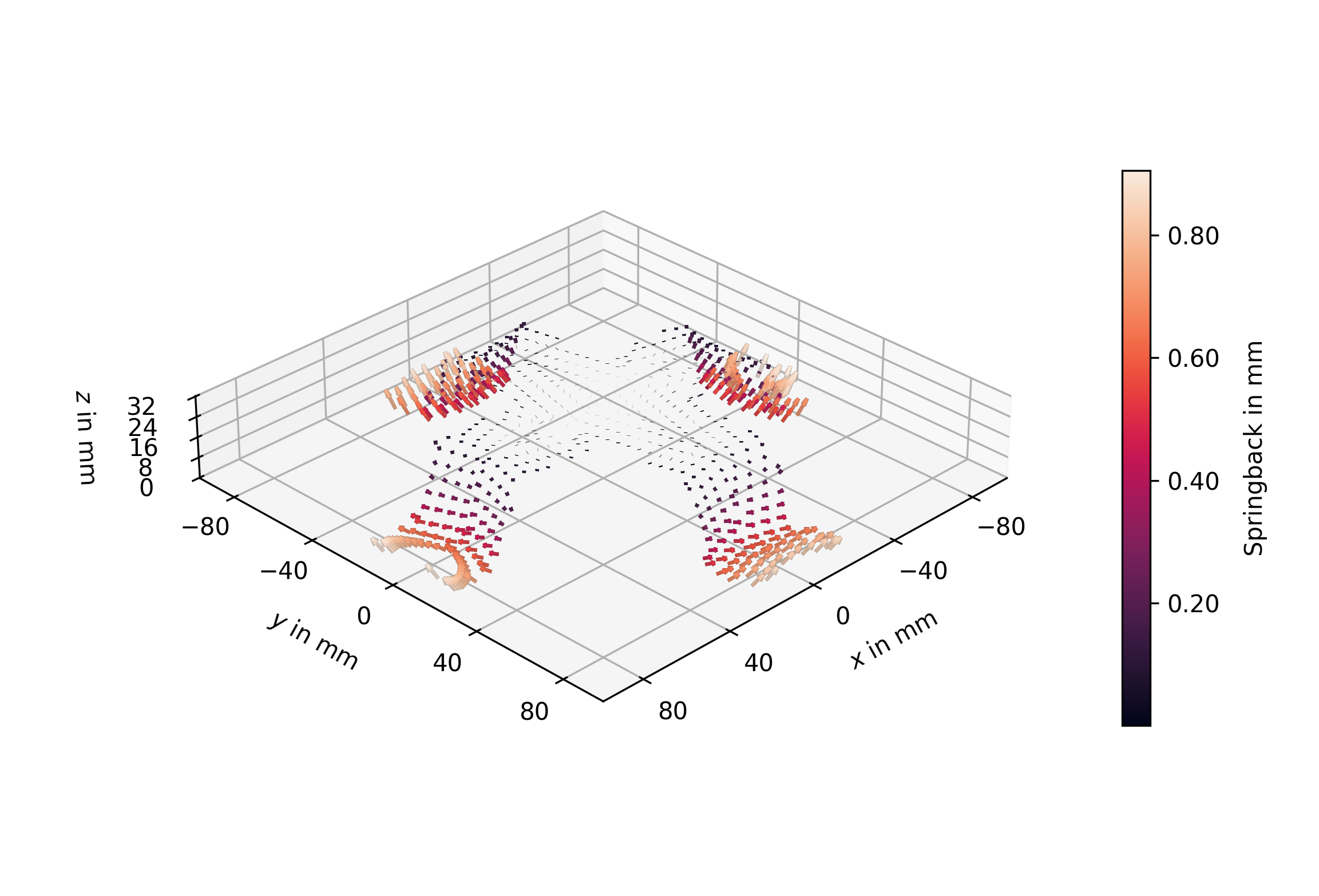
Magnitude alone hides direction: a node that springs radially inward looks the same as one that drops vertically. plot_vectors renders the per-node delta as arrows, so both the local magnitude (arrow colour) and the local direction (arrow vector) are visible.
plot_vectors is a pure arrow renderer. It does not draw an underlying point cloud or mesh. Passing values=magnitude colours each arrow by the springback and builds a matching colorbar. step thins the arrow density so the field stays readable. The default rendering draws a thin black outline behind each arrow (configurable via outline_kwargs, suppress with outline_kwargs={'linewidth': 0}).
ax, cbar = ddacs.plot_vectors(
    pos[-1],
    displacement,
    values=magnitude,
    step=25,
    scale=10.0,
    cmap=ROCKET,
    colorbar_label='Springback in mm',
    mirror=True,
)
plt.show()
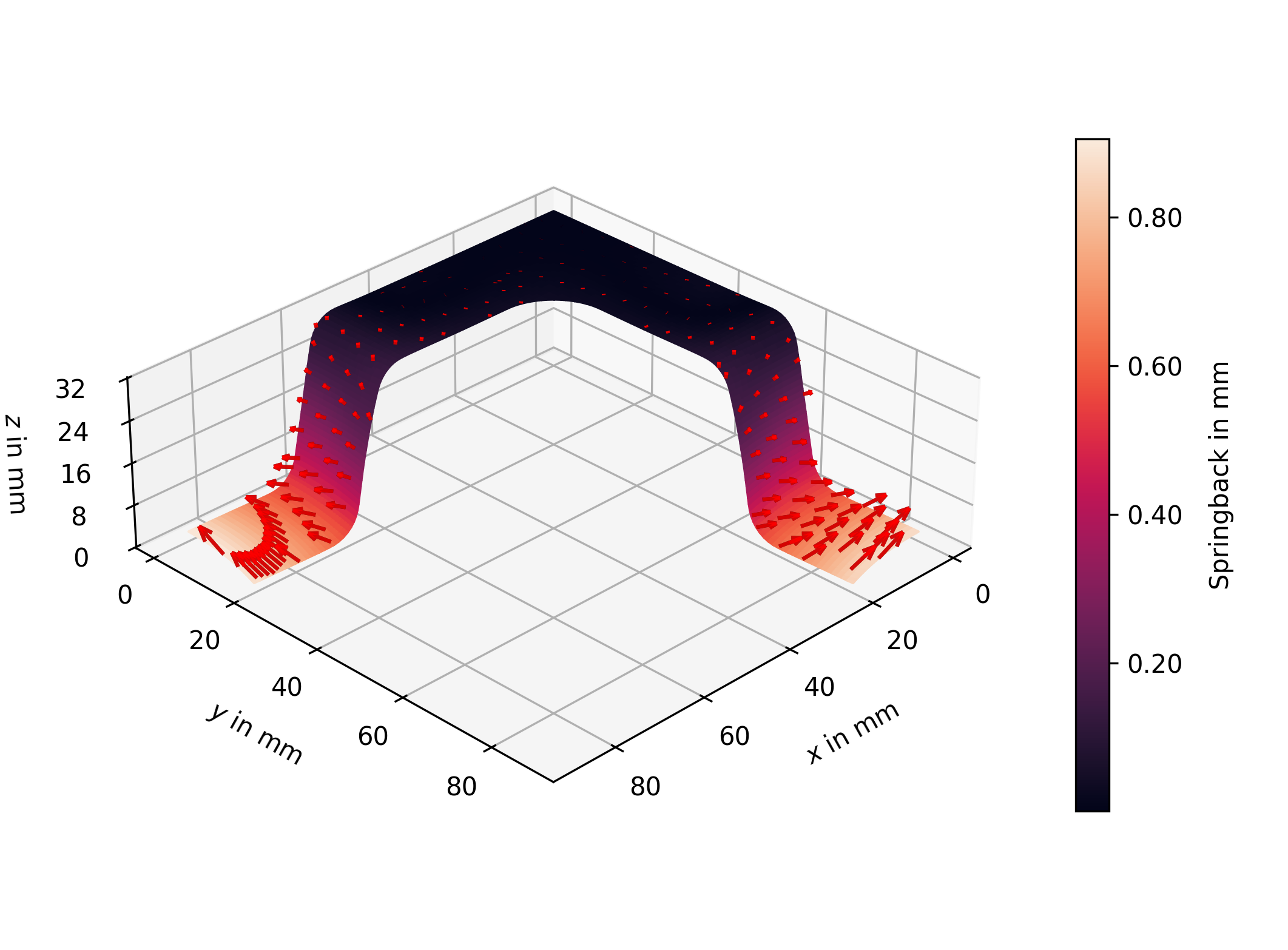
5. Compose: arrows on a coloured mesh
Sections 3 and 4 each show one aspect of the springback: magnitude on a mesh (Section 3) or magnitude plus direction on arrows (Section 4). They can be combined on the same axis to convey both at once. The mesh carries the magnitude (rocket cmap); the arrows carry the direction.
Because plot_mesh, plot_point_cloud, and plot_vectors all accept an existing ax, composition is just two calls in sequence. Solid red arrows are chosen on top so they read as overlay glyphs and do not duplicate the rocket signal already on the mesh.
fig = plt.figure(figsize=(8, 6))
ax  = fig.add_subplot(111, projection='3d')

ddacs.plot_mesh(
    pos[-1], faces20,
    values=face_magnitude,
    ax=ax,
    cmap=ROCKET,
    vmin=float(magnitude.min()),
    vmax=float(magnitude.max()),
    colorbar_label='Springback in mm',
    mirror=False,
    shade=False,
)
# Mesh already encodes magnitude. Arrows in solid red just convey direction.
ddacs.plot_vectors(
    pos[-1],
    displacement,
    ax=ax,
    step=25,
    scale=10.0,
    arrow_kwargs={'color': 'red'},
    mirror=False,
)
plt.show()
For the full function signatures see the Visualization API reference.